Statistical Machine Learning class, STAT-427/627, Dr. M. Baron

PRINCIPAL COMPONENTS AND PARTIAL LEAST SQUARES

1. Eigenvalues and eigenvectors. Spectral decomposition.

> attach(Auto);

> library(ISLR2); attach(Auto);

> X = model.matrix( mpg ~ weight + horsepower + cylinders - 1, data=Auto )

> A = cor(X)

> A

weight horsepower cylinders

weight 1.0000000 0.8645377 0.8975273

horsepower 0.8645377 1.0000000 0.8429834

cylinders 0.8975273 0.8429834 1.0000000

> eigen(A) # This produces eigenvalues and eigenvectors

eigen() decomposition

$values

[1] 2.73689293 0.16323918 0.09986789

$vectors

[,1] [,2] [,3]

[1,] -0.5829268 0.2531535 0.7720813

[2,] -0.5708026 -0.8038435 -0.1673921

[3,] -0.5782566 0.5382834 -0.6130826

> lambda = eigen(A)$values

> Q = eigen(A)$vectors

> # Check QQ' = Q'Q = I and the spectral decomposition

> Q %*% t(Q)

[,1] [,2] [,3]

[1,] 1.000000e+00 5.551115e-17 2.220446e-16

[2,] 5.551115e-17 1.000000e+00 8.326673e-17

[3,] 2.220446e-16 8.326673e-17 1.000000e+00

> t(Q) %*% Q

[,1] [,2] [,3]

[1,] 1.000000e+00 -5.551115e-17 -1.110223e-16

[2,] -5.551115e-17 1.000000e+00 1.665335e-16

[3,] -1.110223e-16 1.665335e-16 1.000000e+00

> # These are identity matrices, all off-diagonal elements are practically 0

> LAMBDA = diag(lambda) # Diagonal matrix with eigenvalues on the diagonal

> lambda

[1] 2.73689293 0.16323918 0.09986789

> LAMBDA

[,1] [,2] [,3]

[1,] 2.736893 0.0000000 0.00000000

[2,] 0.000000 0.1632392 0.00000000

[3,] 0.000000 0.0000000 0.09986789

> Q %*% LAMBDA %*% t(Q) # Spectral decomposition of matrix A

[,1] [,2] [,3]

[1,] 1.0000000 0.8645377 0.8975273

[2,] 0.8645377 1.0000000 0.8429834

[3,] 0.8975273 0.8429834 1.0000000

> A

weight horsepower cylinders

weight 1.0000000 0.8645377 0.8975273

horsepower 0.8645377 1.0000000 0.8429834

cylinders 0.8975273 0.8429834 1.0000000

> # This is the same matrix: Q %*% LAMBDA %*% t(Q) = A.

2. Principal Components

# Let’s investigate the principal components, and how much variance they explain.

> X = model.matrix( mpg ~ .-name-origin+as.factor(origin), data=Auto )

> pc = princomp(X)

> summary(pc)

Importance of components:

Comp.1 Comp.2 Comp.3 Comp.4 Comp.5

Standard deviation 854.5664182 38.860050688 1.614144e+01 3.309297e+00 1.694518e+00

Proportion of Variance 0.9975617 0.002062789 3.559039e-04 1.495959e-05 3.922297e-06

Cumulative Proportion 0.9975617 0.999624521 9.999804e-01 9.999954e-01 9.999993e-01

Comp.6 Comp.7 Comp.8 Comp.9

Standard deviation 5.242357e-01 4.162175e-01 2.443204e-01 1.110223e-16

Proportion of Variance 3.754062e-07 2.366403e-07 8.153944e-08 1.683715e-38

Cumulative Proportion 9.999997e-01 9.999999e-01 1.000000e+00 1.000000e+00

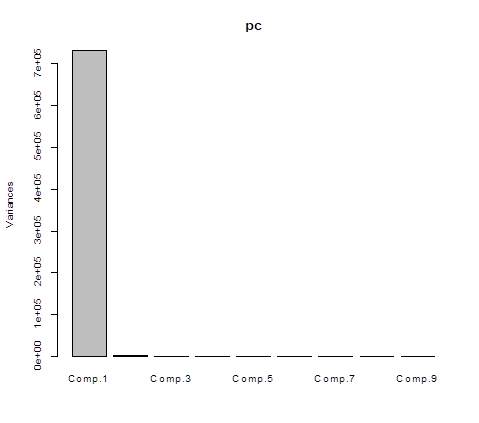
# So, Z₁, the first PC, contains 99.76% of the total variation of X variables. The first two PCs together contain 99.96%. Here is a plot of these percents called a screeplot.

> screeplot(pc)

# The actual coefficients can be obtained by prcomp().

> prcomp(X)

PC1 PC2 PC3 PC4 PC5

(Intercept) 0.0000000000 0.0000000000 0.000000000 0.000000000 0.000000e+00

cylinders -0.0017926225 0.0133245279 -0.007294275 0.001414710 1.719368e-02

displacement -0.1143412856 0.9457785881 -0.303312504 -0.009143349 -1.059355e-02

horsepower -0.0389670412 0.2982553337 0.948761071 -0.043076559 -8.646402e-02

weight -0.9926735354 -0.1207516411 -0.002454212 0.001480458 3.152970e-03

acceleration 0.0013528348 -0.0348264293 -0.077006895 0.059516278 -9.944974e-01

year 0.0013368415 -0.0238516081 -0.042819254 -0.996935229 -5.549653e-02

as.factor(origin)2 0.0001308250 -0.0024889942 0.002857670 0.022100094 -9.052576e-05

as.factor(origin)3 0.0002103564 -0.0003765828 0.004796684 -0.012089823 -1.150938e-03

PC6 PC7 PC8 PC9

(Intercept) 0.0000000000 0.0000000000 0.000000e+00 1

cylinders 0.9911554803 0.1211162208 -4.909265e-02 0

displacement -0.0146594359 -0.0006512752 4.394368e-03 0

horsepower 0.0038232742 0.0034425206 -4.435100e-03 0

weight -0.0002093216 -0.0003053766 5.729471e-06 0

acceleration 0.0168319859 0.0012233398 -1.799780e-03 0

year -0.0001647840 0.0240346554 7.643176e-03 0

as.factor(origin)2 -0.0483462982 0.6888706846 7.229226e-01 0

as.factor(origin)3 0.1214929883 -0.7142804151 6.891098e-01 0

Standardized scale

So, we see that the 1st principal component contains a huge portion of the total variation of X variables, and it is dominated by variable “weight”. Of course! Looking at the data, we see that weight simply has the largest values.

> head(Auto)

mpg cylinders displacement horsepower weight acceleration year origin

1 18 8 307 130 3504 12.0 70 1

2 15 8 350 165 3693 11.5 70 1

3 18 8 318 150 3436 11.0 70 1

4 16 8 304 150 3433 12.0 70 1

5 17 8 302 140 3449 10.5 70 1

6 15 8 429 198 4341 10.0 70 1

# For this reason, usually, X variables are standardized first (subtract each X-variable’s mean and divide by the standard deviation).

> pcr.fit = pcr( mpg ~ .-name-origin+as.factor(origin), data=Auto, scale=TRUE )

> summary(pcr.fit)

TRAINING: % variance explained

1 comps 2 comps 3 comps 4 comps 5 comps 6 comps 7 comps 8 comps

X 56.9 73.02 84.29 92.38 97.29 98.86 99.59 100.00

mpg 71.8 73.64 73.96 79.25 79.25 80.22 81.55 82.42

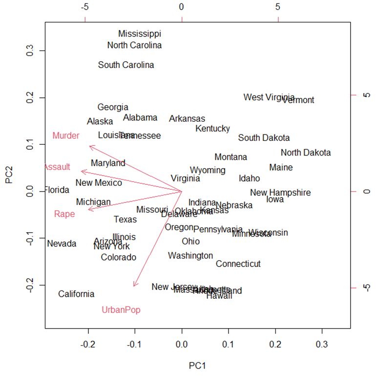
Visualization

> names(USArrests)

[1] "Murder" "Assault" "UrbanPop" "Rape"

> pc = prcomp(USArrests, scale=TRUE)

> biplot(pc)

A map of states with red lines

Description automatically generated with medium confidence

3. Principal Components Regression

> library(pls)

> pcr.fit = pcr( mpg ~ . - name - origin + as.factor(origin), data=Auto )

# Using all variables except name

> summary(pcr.fit)

TRAINING: % variance explained

1 comps 2 comps 3 comps 4 comps 5 comps 6 comps 7 comps 8 comps

X 99.76 99.96 100.00 100.00 100.00 100.00 100.00 100.00

mpg 69.35 70.09 70.75 80.79 80.88 80.91 80.93 82.42

# The “X” row shows % of X variation contained in the given number of PCs.

# The “mpg” row shows R² (% of Y variation explained) from the PC regression. The usual linear regression on all 8 variables has the same R²as PCR that uses all 8 principal components.

> reg = lm( mpg ~ .-name-origin+as.factor(origin), data=Auto )

> summary(reg)

Multiple R-squared: 0.8242

Cross-validation

# Cross-validation. Option validation="CV" does a K-fold cross-validation with K=10, for LOOCV, use validation="LOO".

> pcr.fit = pcr( mpg ~ .-name-origin+as.factor(origin), data=Auto, scale=TRUE, validation="CV" )

> summary(pcr.fit)

VALIDATION: RMSEP

Cross-validated using 10 random segments.

(Intercept) 1 comps 2 comps 3 comps 4 comps 5 comps 6 comps 7 comps 8 comps

CV 7.815 4.162 4.036 4.028 3.611 3.616 3.537 3.427 3.350

adjCV 7.815 4.161 4.034 4.026 3.607 3.613 3.533 3.422 3.346

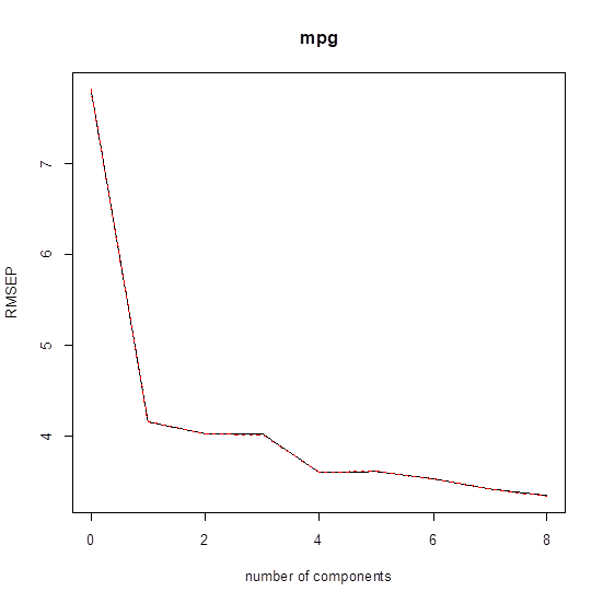
# The predicted error (by cross-validation) is minimized by using all M=8 principal components.

# We can see the graph of root mean-squared error of prediction (or specify val.type)

> validationplot(pcr.fit)

3. Partial Least Squares

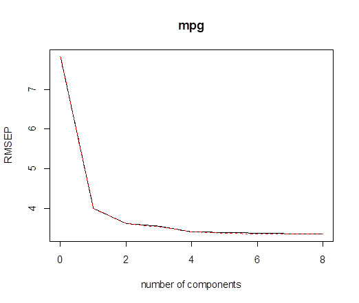
# Similar commands, just replace “pcr” with “plsr”. M=6 components gives the lowest prediction MSE.

> pls = plsr( mpg ~ .-name-origin+as.factor(origin), data=Auto, scale=TRUE, validation="CV" )

> summary(pls)

Cross-validated using 10 random segments.

(Intercept) 1 comps 2 comps 3 comps 4 comps 5 comps 6 comps 7 comps 8 comps

CV 7.815 3.994 3.616 3.540 3.395 3.379 3.351 3.364 3.362

adjCV 7.815 3.992 3.612 3.535 3.390 3.376 3.345 3.359 3.357

TRAINING: % variance explained

1 comps 2 comps 3 comps 4 comps 5 comps 6 comps 7 comps 8 comps

X 56.73 68.84 80.75 84.08 93.48 94.88 99.33 100.00

mpg 74.32 79.37 80.29 81.71 82.00 82.35 82.38 82.42

> validationplot(pls)

# Next, we can fit a model with the desired number of principal components, obtain predicted values, and calculate the prediction mean-squared error. For example:

> n = length(mpg);

> Z = sample(n,n/2);

> PLS = plsr( mpg ~ .-name-origin+as.factor(origin), data=Auto[Z,], scale=TRUE, ncomp=6 );

> Yhat = predict( PLS, newdata=Auto[-Z,], ncomp=6 )

> MSE = mean((Yhat - mpg[-Z])^2)

> MSE

[1] 9.619134

> RMSE = sqrt(MSE)

> RMSE

[1] 3.101473